Using NN’s for Long-Range Forecasts: Electricity Data
In this example we’ll show how to handle complex series. The domain here is electricity-usage data (using a dataset from the UCI Machine Learning Data Repository), and it’s a great example of a challenge for traditional forecasting applications. In these traditional approaches, we divide our model into siloed processes that each contribute to separate behaviors of the time-series. For example:
Hour-in-day effects
Day-in-week effects
Season-in-year effects
Weather effects
However, with electricity data, it’s limiting to model these separately, because these effects all interact: the impact of hour-in-day depends on the day-of-week, the impact of the day-of-week depends on the season of the year, etc.
[2]:
BASE_DIR = 'electricity'
SPLIT_DT = np.datetime64('2013-06-01')
DEVICE = torch.device('cuda' if torch.cuda.is_available() else 'cpu')
Data-Prep
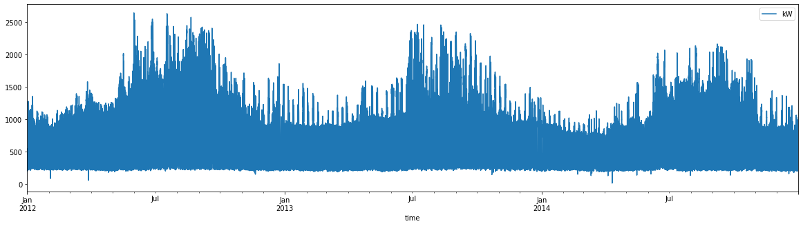
Our dataset consists of hourly kW readings for multiple buildings:
[4]:
df_elec.head()
[4]:
| group | time | kW | dataset | |
|---|---|---|---|---|
| 0 | MT_001 | 2012-01-01 00:00:00 | 3.172589 | train |
| 1 | MT_001 | 2012-01-01 01:00:00 | 4.124365 | train |
| 2 | MT_001 | 2012-01-01 02:00:00 | 4.758883 | train |
| 3 | MT_001 | 2012-01-01 03:00:00 | 4.441624 | train |
| 4 | MT_001 | 2012-01-01 04:00:00 | 4.758883 | train |
Let’s pick an example group to focus on, for demonstration:
[5]:
example_group = 'MT_358'
[6]:
df_elec.query(f"group=='{example_group}'").plot('time', 'kW', figsize=(20, 5))
[6]:
<Axes: xlabel='time'>
[7]:
# we'll apply a sqrt transformation and center before training, and inverse these for plotting/eval:
group_means = (df_elec
               .assign(kW_sqrt = lambda df: np.sqrt(df['kW']))
               .query("dataset=='train'")
               .groupby('group')
               ['kW_sqrt'].mean()
               .to_dict())

def add_transformed(df: pd.DataFrame) -> pd.DataFrame:
    return df.assign(kW_sqrt_c = lambda df: np.sqrt(df['kW']) - df['group'].map(group_means))

def add_inv_transformed(df: pd.DataFrame) -> pd.DataFrame:
    df = df.copy()
    cols = [c for c in ['lower', 'upper', 'mean', 'actual'] if c in df.columns]
    df[cols] += df['group'].map(group_means).to_numpy()[:, None]
    df[cols] = df[cols].clip(lower=0) ** 2
    if 'measure' in df.columns:
        df['measure'] = df['measure'].str.replace('_sqrt_c', '')
    return df
[8]:
df_elec = add_transformed(df_elec)
A Standard Forecasting Approach
First, let’s try a standard exponential-smoothing algorithm on one of the series.
[9]:
from torchcast.process import LocalTrend, Season

es = ExpSmoother(
    measures=['kW_sqrt_c'],
    processes=[
        # seasonal processes:
        Season(id='day_in_week', period=24 * 7, dt_unit='h', K=3, fixed=True),
        Season(id='day_in_year', period=24 * 365.25, dt_unit='h', K=8, fixed=True),
        Season(id='hour_in_day', period=24, dt_unit='h', K=8, fixed=True),
        # long-running trend:
        LocalTrend(id='trend'),
    ]
)
[10]:
ds_example_building = TimeSeriesDataset.from_dataframe(
    df_elec.query("group == @example_group"),
    group_colname='group',
    time_colname='time',
    dt_unit='h',
    measure_colnames=['kW_sqrt_c'],
)
ds_example_train, _ = ds_example_building.train_val_split(dt=SPLIT_DT)
ds_example_train
[10]:
TimeSeriesDataset(sizes=[torch.Size([1, 12408, 1])], measures=(('kW_sqrt_c',),))
[11]:
es.fit(
    ds_example_train.tensors[0],
    start_offsets=ds_example_train.start_datetimes,
)
For measure kW_sqrt_c, setting initial value by setting 'trend.position' to -0.0000
[11]:
ExpSmoother(
  (measure_covariance): Covariance()
  (processes): ModuleDict(
    (day_in_week): Season(id='day_in_week', measure='kW_sqrt_c')
    (day_in_year): Season(id='day_in_year', measure='kW_sqrt_c')
    (hour_in_day): Season(id='hour_in_day', measure='kW_sqrt_c')
    (trend): LocalTrend(id='trend', measure='kW_sqrt_c')
  )
  (smoothing_matrix): SmoothingMatrix()
)
Visualizing the results is… not that illuminating:
[12]:
es_predictions = es(
    ds_example_train.tensors[0],
    start_offsets=ds_example_train.start_datetimes,
    # note we're *not* getting `num_timesteps` from `ds_example_train`, since we want to forecast outside the training time:
    out_timesteps=ds_example_building.num_timesteps
)
es_predictions.plot(es_predictions.to_dataframe(ds_example_train), split_dt=SPLIT_DT)
/Users/jacobdink/miniconda3/envs/torchcast/lib/python3.9/site-packages/plotnine/geoms/geom_path.py:100: PlotnineWarning: geom_path: Removed 13896 rows containing missing values.
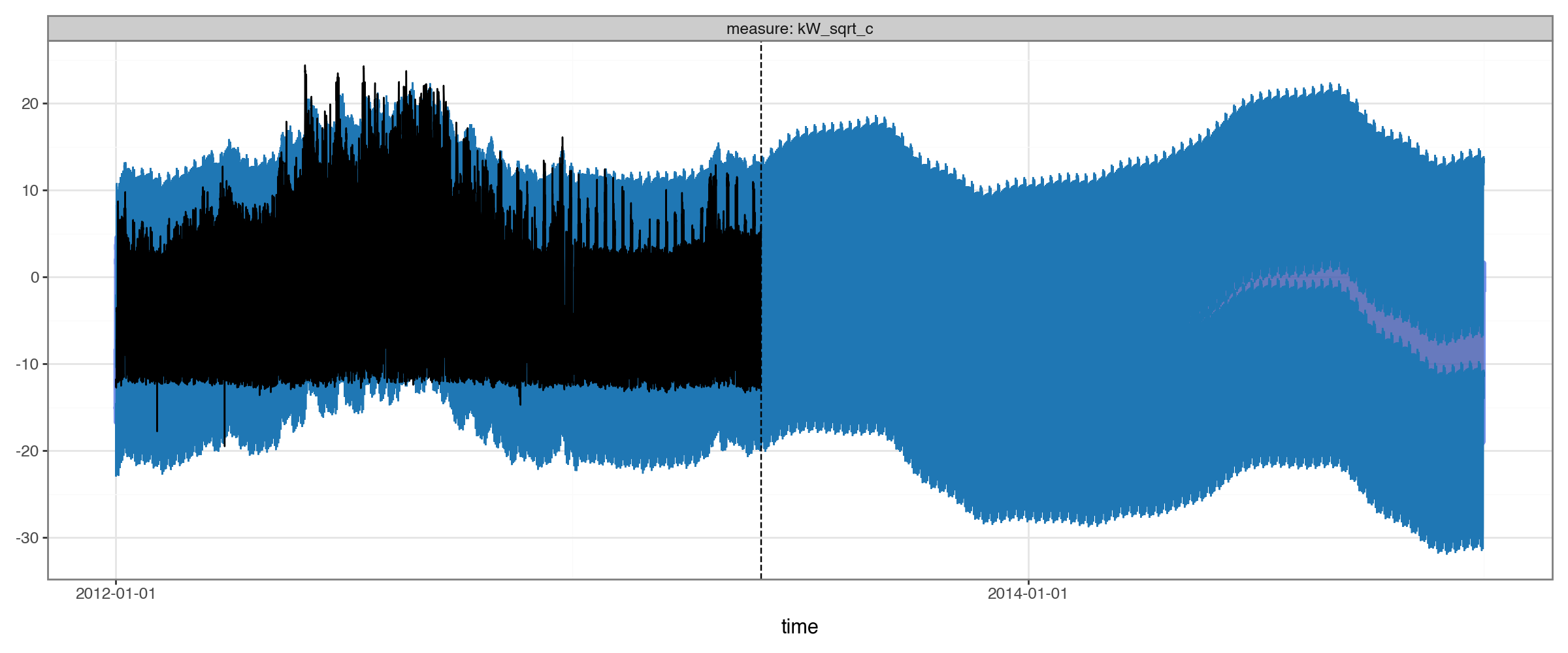
With hourly data, it’s just really hard to see the data when we are this zoomed out!
We can try zooming in:
[13]:
es_predictions.plot(
    es_predictions
    .to_dataframe(ds_example_building).query("time.between('2013-05-15', '2013-06-15')")
    .pipe(add_inv_transformed),
    split_dt=SPLIT_DT
)
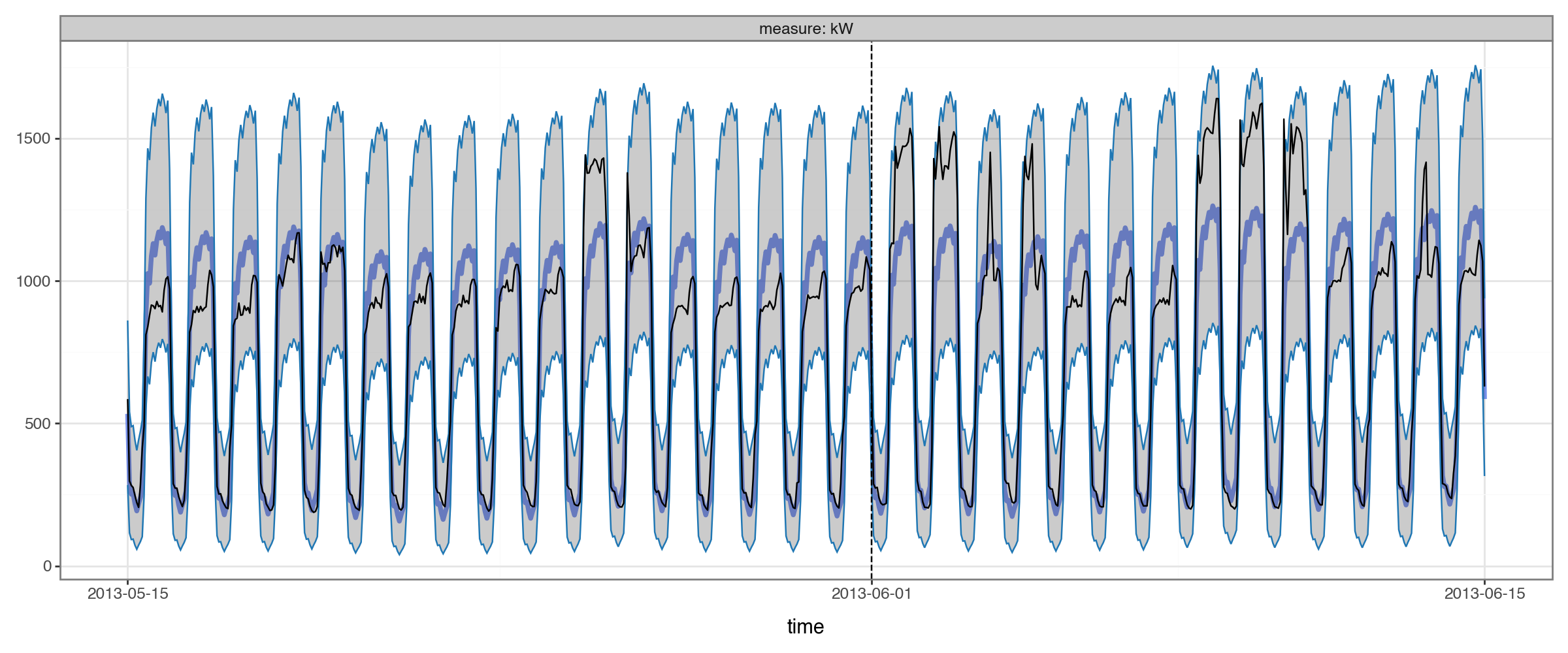
This is better for actually seeing the data, but ideally we’d still like to get a view of the long range.
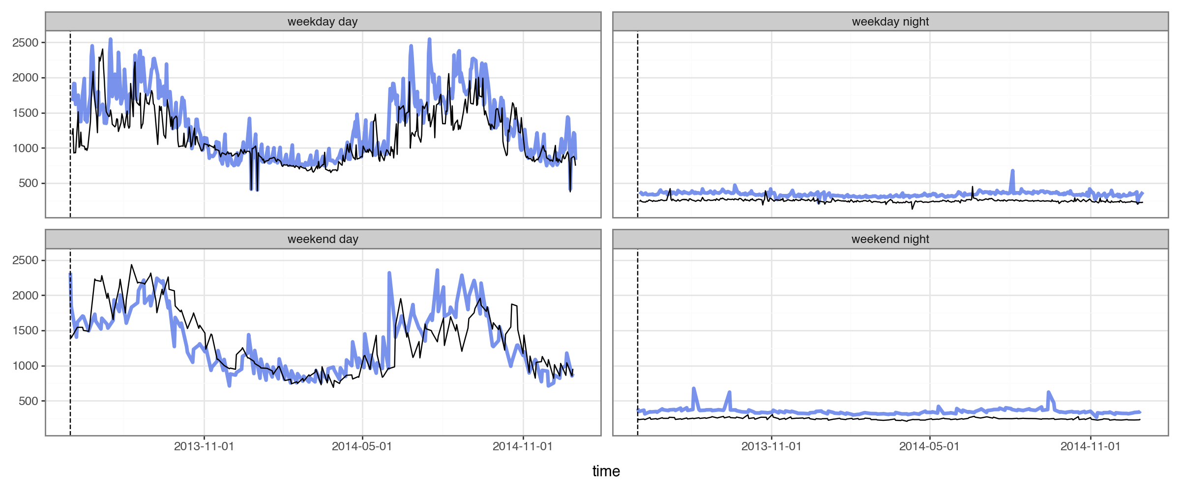
Let’s instead try splitting it into weekdays vs. weekends and daytimes vs. nightimes:
[14]:
def plot_2x2(df: pd.DataFrame,
             pred_colname: str = 'mean',
             actual_colname: str = 'actual',
             group_colname: str = 'group',
             time_colname: str = 'time',
             **kwargs):
    """
    Plot predicted vs. actual for a single group, splitting into 2x2 facets of weekday/end * day/night.
    """
    df_plot = df.assign(
        time_of_day=None,
        weekend=lambda df: np.where(df[time_colname].dt.weekday.isin([5, 6]), 'weekend', 'weekday'),
        date=lambda df: df[time_colname].dt.normalize()
    )
    df_plot.loc[df_plot[time_colname].dt.hour.isin([14, 15, 16, 17, 18]), 'time_of_day'] = 'day'
    df_plot.loc[df_plot[time_colname].dt.hour.isin([2, 3, 4, 5, 6]), 'time_of_day'] = 'night'
    df_plot[time_colname] = df_plot.pop('date')
    _agg = [pred_colname, actual_colname]
    if 'upper' in df_plot.columns:
        _agg.extend(['upper', 'lower'])
    df_plot = df_plot.groupby([group_colname, time_colname, 'weekend', 'time_of_day'])[_agg].mean().reset_index()
    df_plot['measure'] = df_plot['weekend'] + ' ' + df_plot['time_of_day']
    df_plot['mean'] = df_plot.pop(pred_colname)
    df_plot['actual'] = df_plot.pop(actual_colname)
    if 'upper' not in df_plot.columns:
        df_plot['lower'] = df_plot['upper'] = float('nan')
    return Predictions.plot(df_plot, time_colname=time_colname, group_colname=group_colname, **kwargs) + facet_wrap('measure')
[15]:
plot_2x2(es_predictions
.to_dataframe(ds_example_building)
.pipe(add_inv_transformed)
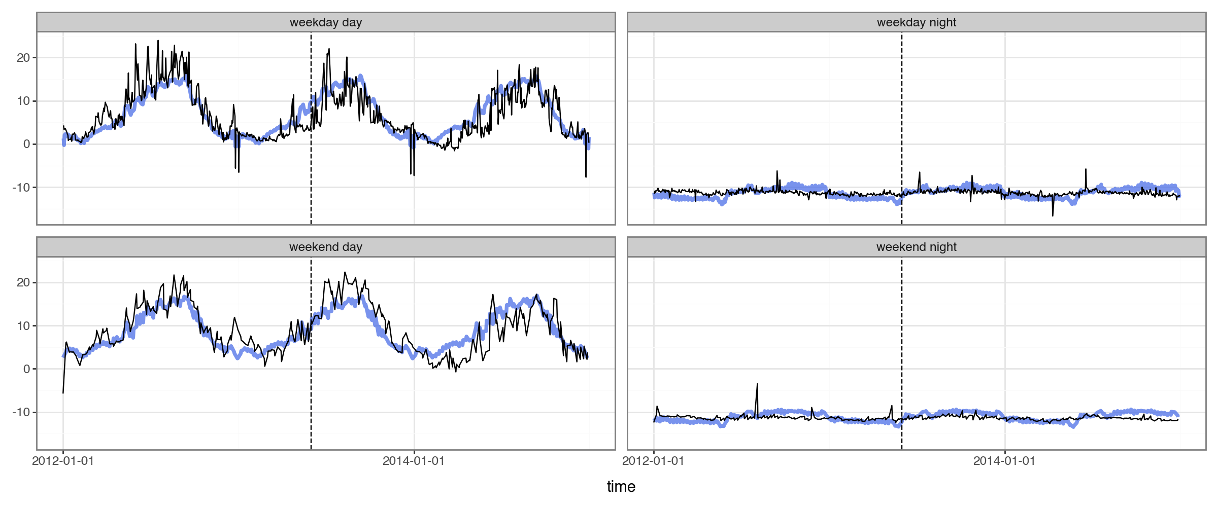
,split_dt=SPLIT_DT)
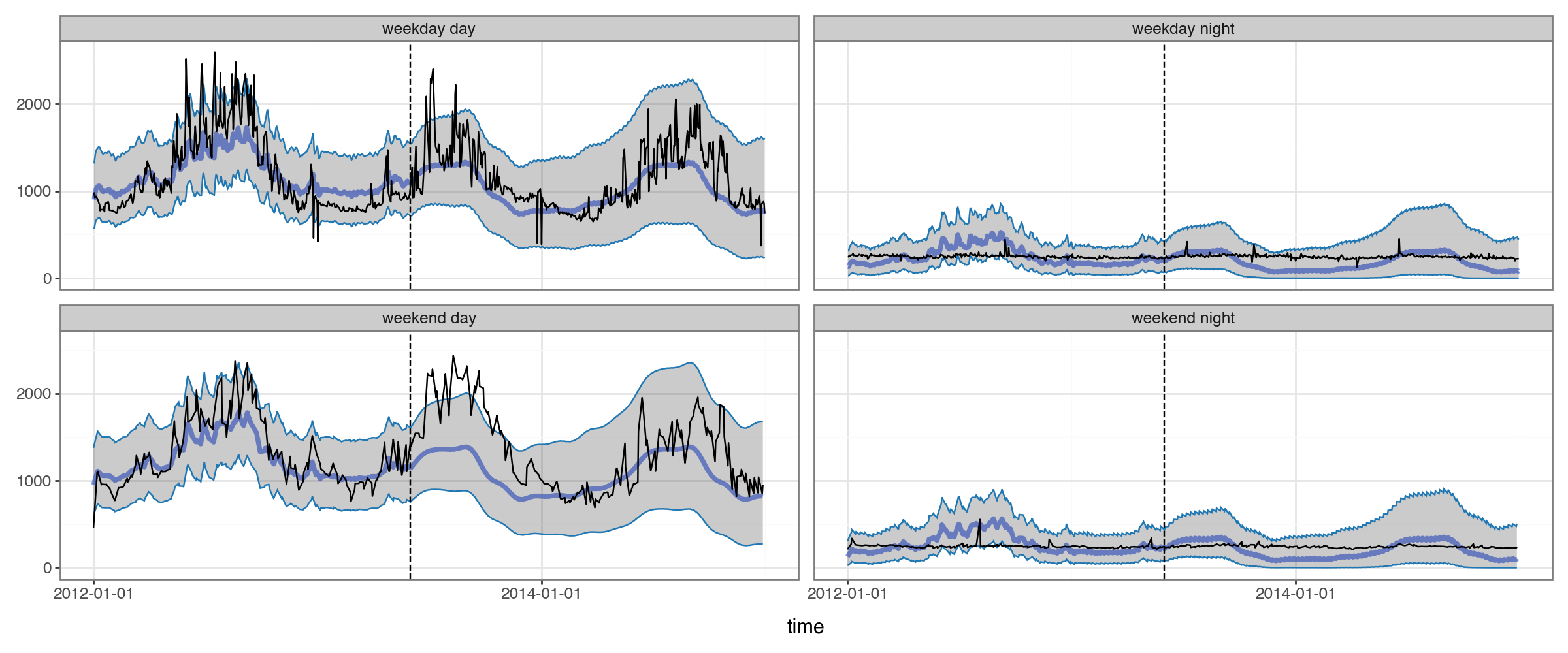
Viewing the forecasts in this way helps us see a serious issue: the annual seasonal pattern is very different for daytimes and nighttimes, but the model isn’t capturing that at all. (In fact, even the lower amplitude in annual seasonality for nighttime forecasts is just an artifact of our sqrt-transform, not a product of the model.)
The limitation is inherent to the model: it only allows for a single seasonal pattern, rather than a separate one for different times of the day and days of the week.
Incorporating a Neural Network
We saw our model wasn’t allowing for interactions among the components of the time-series. A natural solution to this is to incorporate a neural network – learning arbitrary/complex interactions is exactly what they are for.
Of course, this requires scaling up our dataset: we want to learn across multiple series, so that our network can build representations of patterns that are shared across multiple buildings.
Encoding Seasonlity as Fourier Terms
We’re going to need to encode the seasonal cycles in our data into features that a neural-network can use as inputs.
There are multiple ways we can do this. For example, one option would be to extract each component of our datetimes and one-hot encode it:
[16]:
(df_elec
 .loc[df_elec['group']==example_group,['time']]
 .assign(hod=lambda df: df['time'].dt.hour, dow=lambda df: df['time'].dt.dayofweek)
 .pipe(pd.get_dummies, columns=['hod', 'dow'], dtype='float')
 .head())
[16]:
| time | hod_0 | hod_1 | hod_2 | hod_3 | hod_4 | hod_5 | hod_6 | hod_7 | hod_8 | ... | hod_21 | hod_22 | hod_23 | dow_0 | dow_1 | dow_2 | dow_3 | dow_4 | dow_5 | dow_6 | |
|---|---|---|---|---|---|---|---|---|---|---|---|---|---|---|---|---|---|---|---|---|---|
| 9232450 | 2012-01-01 00:00:00 | 1.0 | 0.0 | 0.0 | 0.0 | 0.0 | 0.0 | 0.0 | 0.0 | 0.0 | ... | 0.0 | 0.0 | 0.0 | 0.0 | 0.0 | 0.0 | 0.0 | 0.0 | 0.0 | 1.0 |
| 9232451 | 2012-01-01 01:00:00 | 0.0 | 1.0 | 0.0 | 0.0 | 0.0 | 0.0 | 0.0 | 0.0 | 0.0 | ... | 0.0 | 0.0 | 0.0 | 0.0 | 0.0 | 0.0 | 0.0 | 0.0 | 0.0 | 1.0 |
| 9232452 | 2012-01-01 02:00:00 | 0.0 | 0.0 | 1.0 | 0.0 | 0.0 | 0.0 | 0.0 | 0.0 | 0.0 | ... | 0.0 | 0.0 | 0.0 | 0.0 | 0.0 | 0.0 | 0.0 | 0.0 | 0.0 | 1.0 |
| 9232453 | 2012-01-01 03:00:00 | 0.0 | 0.0 | 0.0 | 1.0 | 0.0 | 0.0 | 0.0 | 0.0 | 0.0 | ... | 0.0 | 0.0 | 0.0 | 0.0 | 0.0 | 0.0 | 0.0 | 0.0 | 0.0 | 1.0 |
| 9232454 | 2012-01-01 04:00:00 | 0.0 | 0.0 | 0.0 | 0.0 | 1.0 | 0.0 | 0.0 | 0.0 | 0.0 | ... | 0.0 | 0.0 | 0.0 | 0.0 | 0.0 | 0.0 | 0.0 | 0.0 | 0.0 | 1.0 |
5 rows × 32 columns
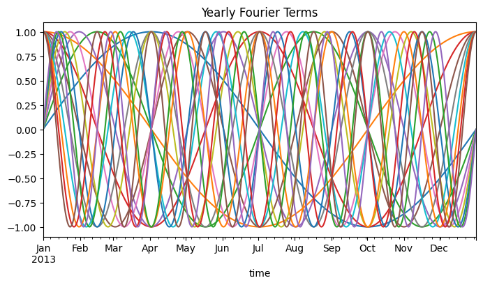
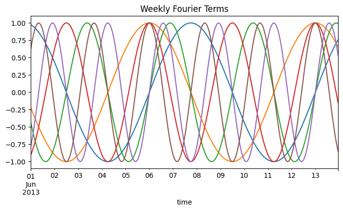
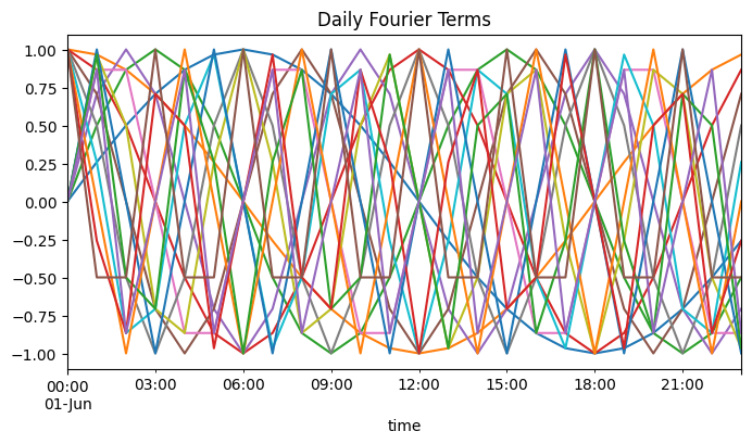
Instead, we’ll use a different approach based on fourier series. Basically, we encoded our times into sine/cosine waves. The number of waves is a hyper-parameter that can be tuned and helps us control how ‘wiggly’ we’ll allow the seasons to be. For more reading on using fourier series for modeling seasonality, see here and here.
For visualizing this (and shortly, for modeling), we’ll use torchcast’s add_season_features function:
[17]:
from torchcast.utils import add_season_features

df_example = (df_elec[df_elec['group'] == example_group]
              .reset_index(drop=True)
              .pipe(add_season_features, K=8, period='yearly')
              .pipe(add_season_features, K=3, period='weekly')
              .pipe(add_season_features, K=8, period='daily'))

yearly_season_feats = df_example.columns[df_example.columns.str.startswith('yearly_')].tolist()
weekly_season_feats = df_example.columns[df_example.columns.str.startswith('weekly_')].tolist()
daily_season_feats = df_example.columns[df_example.columns.str.startswith('daily_')].tolist()
season_feats = yearly_season_feats + weekly_season_feats + daily_season_feats
[18]:
(df_example[yearly_season_feats + ['time']]
 .query("time.dt.year == 2013")
 .plot(x='time', figsize=(8,4), legend=False, title='Yearly Fourier Terms'))

(df_example[weekly_season_feats + ['time']]
 .query("(time.dt.year == 2013) & (time.dt.month == 6) & (time.dt.day < 14)")
 .plot(x='time', figsize=(8,4), legend=False, title='Weekly Fourier Terms'))

(df_example[daily_season_feats + ['time']]
 .query("(time.dt.year == 2013) & (time.dt.month == 6) & (time.dt.day == 1)")
 .plot(x='time', figsize=(8,4), legend=False, title='Daily Fourier Terms'))
[18]:
<Axes: title={'center': 'Daily Fourier Terms'}, xlabel='time'>
Step 1: Pre-Training a Seasonal-Embeddings NN
For this task, we’ll switch from exponential smoothing (with ExpSmoother) to a full state-space model (with KalmanFilter). This is because only the latter can learn relationships specific to each time-series.
The LinearModel provides a catch-all for any way of passing arbitrary inputs to our model. For example, if we had weather data – temperature, humidity, wind-speed – we might add a process like:
LinearModel(id='weather', predictors=['temp','rhumidity','windspeed'])
And our time-series model would learn how each of these impacts our series(es).
Here we are using LinearModel a little differently: rather than it taking as input predictors, it will take as input the output of a neural-network, which itself will take predictors (the calendar-features we just defined).
What we’d like to do is train a neural network to embed the seasonality (as represented by our fourier terms) into a lower dimensional space, then we’ll pass that lower dimensional representation onto our KalmanFilter/LinearModel, which will learn how each time-series behaves in relation to that space. Basically, we are reducing the dozens of calendar-features (and their hundreds of interactions) into an efficient low-dimensional representation.
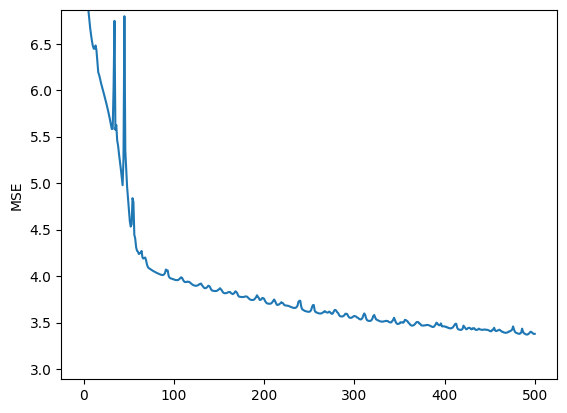
The ModelMatEmbeddingsTrainer class is designed for this kind of use-case. It trains a module to find a lower-dimensional representation of a large model-matrix. Its objective function is how well that lower-dimensional representation works as a linear predictor when we fit a separate linear model to each group (which is similar to what our KalmanFilter will do).
We set up a simple neural network:
[19]:
from torchcast.utils.training import ModelMatEmbeddingsTrainer

SEASON_EMBED_NDIM = 20

season_embedder = torch.nn.Sequential(
    torch.nn.LazyLinear(out_features=48),
    torch.nn.Tanh(),
    torch.nn.Linear(48, 48),
    torch.nn.Tanh(),
    torch.nn.Linear(48, SEASON_EMBED_NDIM)
)
season_trainer = ModelMatEmbeddingsTrainer(season_embedder)
Again, the number of embedding dimensions is a hyper-parameter, where we trade off computational efficiency for precision.
This trainer class expects a TimeSeriesDataLoader, which lets us iterate over the whole dataset in a training loop, yielding each batch as a TimeSeriesDataset.
This TimeSeriesDataLoader class lets us pass a function for the X_colnames argument, so we’ll set that up to create the to-be-reduced fourier features. (Passing a function here is handy since our dataframe is large – it’s more memory-efficient to create the features lazily as each batch is yielded.)
[20]:
def get_season_df(df: pd.DataFrame) -> pd.DataFrame:
    return (df
            .loc[:,['time']]
            .pipe(add_season_features, K=8, period='yearly')
            .pipe(add_season_features, K=3, period='weekly')
            .pipe(add_season_features, K=8, period='daily')
            .drop(columns=['time']))

season_dl = TimeSeriesDataLoader.from_dataframe(
    df_elec.query("dataset=='train'"),
    group_colname='group',
    time_colname='time',
    dt_unit='h',
    y_colnames=['kW_sqrt_c'],
    X_colnames=get_season_df,
    batch_size=45 # fairly even batch sizes
)
Let’s use our trainer:
[21]:
try:
_path = os.path.join(BASE_DIR, f"season_trainer{SEASON_EMBED_NDIM}.pt")
with open(_path, 'rb') as f:
season_trainer = pickle.load(f).to(DEVICE)
season_embedder = season_trainer.module
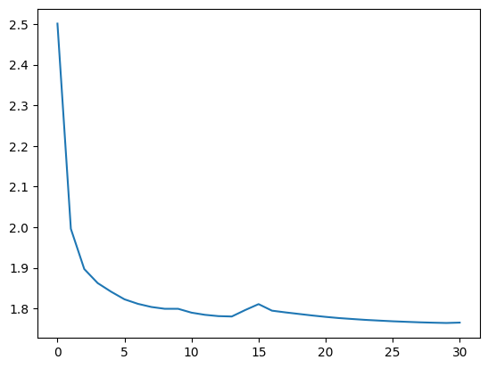
plt.plot(season_trainer.loss_history)
plt.ylim(None, max(season_trainer.loss_history[5:]))
plt.ylabel('MSE')
plt.show()
except FileNotFoundError as e:
from IPython.display import clear_output
season_trainer.loss_history = []
for loss in season_trainer(season_dl):
season_trainer.loss_history.append(loss)
# plot:
if len(season_trainer.loss_history) > 5:
clear_output(wait=True)
plt.plot(season_trainer.loss_history)
plt.ylim(None, max(season_trainer.loss_history[5:]))
plt.ylabel('MSE')
plt.show()
# simple stopping check for this demo
if len(season_trainer.loss_history) > 500:
break
with open(_path, 'wb') as f:
pickle.dump(season_trainer.to(torch.device('cpu')), f)
Let’s visualize the output of this neural network, with each color being a separate output:
[22]:
ds_example2 = TimeSeriesDataset.from_dataframe(
    df_elec
        .query("group == @example_group")
        .pipe(add_season_features, K=8, period='yearly')
        .pipe(add_season_features, K=3, period='weekly')
        .pipe(add_season_features, K=8, period='daily'),
    group_colname='group',
    time_colname='time',
    dt_unit='h',
    y_colnames=['kW_sqrt_c'],
    X_colnames=season_feats
)
[23]:
with torch.no_grad():
    pred = season_embedder(ds_example2.tensors[1])
    _df_pred = pd.DataFrame(pred.squeeze(0).cpu().numpy()).assign(time=ds_example2.times().squeeze(0))

    (_df_pred
         .query("(time.dt.year == 2013) & (time.dt.month == 6) & (time.dt.day < 7)")
         .plot(x='time', figsize=(10,5), legend=False, title=f'Season NN (dim={SEASON_EMBED_NDIM}) Output', alpha=0.5))

    (_df_pred
         .query("(time.dt.year == 2013) & (time.dt.month < 6)")
         .plot(x='time', figsize=(10,5), legend=False, title=f'Season NN (dim={SEASON_EMBED_NDIM}) Output', alpha=0.25))
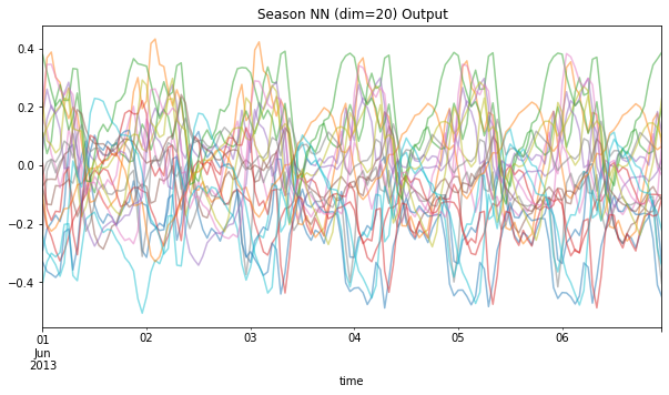

You can think of each colored line as equivalent to the sin/cos waves above; but now, instead of dozens of these, we have far fewer, that should hopefully be able to capture interacting seasonal effects.
Let’s verify this. The season-trainer has a predict method that lets us visualize how these embeddings can be used to predict the actual series values:
[24]:
with torch.no_grad():
    display(ds_example2
             .to_dataframe()
             .assign(pred=season_trainer.predict(ds_example2).cpu().squeeze())
             .pipe(plot_2x2, actual_colname='kW_sqrt_c', pred_colname='pred', split_dt=SPLIT_DT))
Success! We now have different seasonal patterns depending on the time of the day.
Step 2: Incorporate our Seasonal-Embeddings into our Time-Series Model
How should we incorporate our embedding neural-network into a state-space model? First, we create our time-series model:
[25]:
from torchcast.kalman_filter import KalmanFilter
from torchcast.process import LinearModel, LocalLevel

season_embedder.to(DEVICE)

kf_nn = KalmanFilter(
    measures=['kW_sqrt_c'],
    processes=[
        LinearModel(id='nn_output', predictors=[f'nn{i}' for i in range(SEASON_EMBED_NDIM)]),
        LocalLevel(id='level'),
    ],
).to(DEVICE)
Then, we’ll set up another dataloader (with the same function to create the season-features) and another trainer (with instructions on reducing those season features):
[26]:
from torchcast.utils import StateSpaceTrainer

def dataset_to_kwargs(batch: TimeSeriesDataset) -> dict:
    y, seasonX = batch.tensors
    return {'X' : season_embedder(seasonX)}

ss_trainer = StateSpaceTrainer(
    module=kf_nn,
    dataset_to_kwargs=dataset_to_kwargs,
    optimizer=torch.optim.Adam(kf_nn.parameters(), lr=.05)
)
Training End-to-End
Above, we never actually registered season_embedder as an attribute of our KalmanFilter (i.e. we didn’t do kf_nn.season_nn = season_embedder). This means that we won’t continue training the embeddings as we train our KalmanFilter. Why not? For that matter, why did we pre-train in the first place? Couldn’t we have just registered an untrained embeddings network and trained the whole thing end to end?
In practice, neural-networks have many more parameters and take many more epochs than our state-space models (and conversely, our state-space models are much slower to train per epoch). So it’s much more efficient to pre-train the network first. Then it’s up to us whether we want to continue training the network, or just freeze its weights (i.e. exclude it from the optimizer) and just train the state-space models’ parameters. Here we’re freezing them by not assigning the network as an
attribute (so that the parameters don’t get passed to when we run torch.optim.Adam(kf_nn.parameters(), lr=.05)).
[27]:
dataloader_kf_nn = TimeSeriesDataLoader.from_dataframe(
    df_elec.query("dataset=='train'"),
    group_colname='group',
    time_colname='time',
    dt_unit='h',
    y_colnames=['kW_sqrt_c'],
    X_colnames=get_season_df,
    batch_size=45
)
[28]:
try:
    _path = os.path.join(BASE_DIR, f"ss_trainer{SEASON_EMBED_NDIM}_attempt1.pt")
    with open(_path, 'rb') as f:
        ss_trainer = pickle.load(f).to(DEVICE)
    kf_nn = ss_trainer.module
    plt.plot(ss_trainer.loss_history)
    plt.show()
except FileNotFoundError as e:
    torch.cuda.empty_cache()
    ss_trainer.loss_history = []
    for loss in ss_trainer(dataloader_kf_nn, forward_kwargs={'n_step' : 24 * 25, 'every_step' : False}):
        ss_trainer.loss_history.append(loss)
        print(loss)

        with open(_path, 'wb') as f:
            pickle.dump(ss_trainer, f)

        if len(ss_trainer.loss_history) > 30:
            break
Now we’ll create forecasts for all the groups, and back-transform them, for plotting and evaluation.
[29]:
with torch.inference_mode():
    dataloader_all = TimeSeriesDataLoader.from_dataframe(
        # importantly, we'll set to `nan` our target when it's outside the training dates
        # this allows us to use `season_feats` in the forecast period, while not having data-leakage
        df_elec.assign(kW_sqrt_c=lambda df: df['kW_sqrt_c'].where(df['dataset']=='train')),
        group_colname='group',
        time_colname='time',
        dt_unit='h',
        y_colnames=['kW_sqrt_c'],
        X_colnames=get_season_df,
        batch_size=50
    )

    df_all_preds = []
    for batch in tqdm(dataloader_all):
        batch = batch.to(DEVICE)
        X = season_embedder(batch.tensors[1])
        pred = kf_nn(batch.tensors[0], X=X, start_offsets=batch.start_offsets)
        df_all_preds.append(pred.to_dataframe(batch).drop(columns=['actual']))
df_all_preds = pd.concat(df_all_preds).reset_index(drop=True)

# back-transform:
df_all_preds = (df_all_preds
                 .merge(df_elec[['group','time','kW','dataset']])
                 .pipe(add_inv_transformed))
df_all_preds
[29]:
| mean | lower | upper | group | time | measure | kW | dataset | |
|---|---|---|---|---|---|---|---|---|
| 0 | 1.205373 | 0.000000 | 72.527152 | MT_001 | 2012-01-01 00:00:00 | kW | 3.172589 | train |
| 1 | 1.064404 | 0.000000 | 25.518437 | MT_001 | 2012-01-01 01:00:00 | kW | 4.124365 | train |
| 2 | 1.993686 | 0.000000 | 25.204861 | MT_001 | 2012-01-01 02:00:00 | kW | 4.758883 | train |
| 3 | 3.217787 | 0.000000 | 27.541162 | MT_001 | 2012-01-01 03:00:00 | kW | 4.441624 | train |
| 4 | 2.520015 | 0.000000 | 25.331753 | MT_001 | 2012-01-01 04:00:00 | kW | 4.758883 | train |
| ... | ... | ... | ... | ... | ... | ... | ... | ... |
| 9548093 | 936.426328 | 570.241231 | 1392.964735 | MT_369 | 2014-12-31 19:00:00 | kW | 692.631965 | val |
| 9548094 | 899.374697 | 541.382866 | 1347.735523 | MT_369 | 2014-12-31 20:00:00 | kW | 688.416422 | val |
| 9548095 | 860.769343 | 511.492706 | 1300.434453 | MT_369 | 2014-12-31 21:00:00 | kW | 662.023460 | val |
| 9548096 | 873.728189 | 521.490158 | 1316.356523 | MT_369 | 2014-12-31 22:00:00 | kW | 679.252199 | val |
| 9548097 | 886.611285 | 531.450229 | 1332.164842 | MT_369 | 2014-12-31 23:00:00 | kW | 659.274194 | val |
9548098 rows × 8 columns
[30]:
plot_2x2(df_all_preds.query("group==@example_group"), actual_colname='kW', split_dt=SPLIT_DT) #+ scale_y_continuous(trans='log1p')
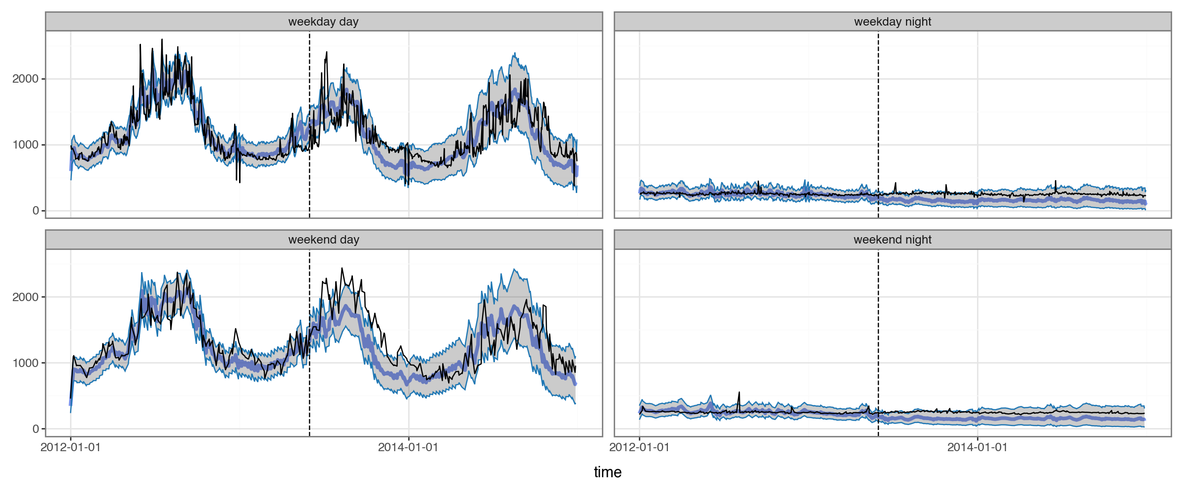
Success! If our example group is representative, our forecasting model was able to use the embeddings to capture complex seasonal structure.
Evaluation
A Simple Baseline
We’ve see that, for this dataset, generating forecasts that are sane is already an achievement.
But of course, ideally we’d actually have some kind of a quantitative measure of how good our forecasts are.
For this, it’s helpful to compare to a baseline. torchcast provides a simple baseline which just forecasts based on N-timesteps ago, with options for first smoothing the historical data. In this case, we forecast based on the same timepoint 365 days ago, after first applying a rolling-average with a 4-hour window.
[31]:
from torchcast.utils import make_baseline

df_baseline365 = make_baseline(df_elec,
                                group_colnames=['group'],
                                time_colname='time',
                                value_colname='kW',
                                is_train=lambda df: df['dataset']=='train',
                                lag=int(365*24),
                                smooth=4)
plot_2x2(
    df_baseline365.query("group==@example_group").merge(df_elec),
    pred_colname='baseline',
    actual_colname='kW',
    split_dt=SPLIT_DT
)
We can see this baseline provides sensible enough forecasts on our example building.
Comparison of Performance
Now that we have something to compare our torchcast model to, we can evaluate its performance.
[32]:
df_compare = (df_all_preds[['group', 'mean', 'time', 'kW', 'dataset']]
             .rename(columns={'mean' : 'torchcast'})
             .merge(df_baseline365, how='left'))

df_compare_long = df_compare.melt(
    id_vars=['group', 'time', 'kW', 'dataset'],
    value_vars=['torchcast', 'baseline'],
    var_name='model',
    value_name='forecast'
)
df_compare_long['error'] = np.abs(df_compare_long['forecast'] - df_compare_long['kW'])
df_compare_long
[32]:
| group | time | kW | dataset | model | forecast | error | |
|---|---|---|---|---|---|---|---|
| 0 | MT_001 | 2012-01-01 00:00:00 | 3.172589 | train | torchcast | 1.205373 | 1.967216 |
| 1 | MT_001 | 2012-01-01 01:00:00 | 4.124365 | train | torchcast | 1.064404 | 3.059961 |
| 2 | MT_001 | 2012-01-01 02:00:00 | 4.758883 | train | torchcast | 1.993686 | 2.765198 |
| 3 | MT_001 | 2012-01-01 03:00:00 | 4.441624 | train | torchcast | 3.217787 | 1.223838 |
| 4 | MT_001 | 2012-01-01 04:00:00 | 4.758883 | train | torchcast | 2.520015 | 2.238868 |
| ... | ... | ... | ... | ... | ... | ... | ... |
| 19096191 | MT_369 | 2014-12-31 19:00:00 | 692.631965 | val | baseline | 712.793255 | 20.161290 |
| 19096192 | MT_369 | 2014-12-31 20:00:00 | 688.416422 | val | baseline | 702.025293 | 13.608871 |
| 19096193 | MT_369 | 2014-12-31 21:00:00 | 662.023460 | val | baseline | 708.486070 | 46.462610 |
| 19096194 | MT_369 | 2014-12-31 22:00:00 | 679.252199 | val | baseline | 728.464076 | 49.211877 |
| 19096195 | MT_369 | 2014-12-31 23:00:00 | 659.274194 | val | baseline | 751.282991 | 92.008798 |
19096196 rows × 7 columns
Over Time
First let’s compare abs(error) over time, across all groups:
[33]:
df_compare_per_date = (df_compare_long
                       .query("dataset!='train'")
                       .assign(date=lambda df: df['time'].dt.normalize())
                       .groupby(['date', 'model'])
                       ['error'].mean()
                       .reset_index())
(df_compare_per_date
 .pivot(index='date', columns='model', values='error')
 .plot(ylim=(0, 300), ylabel="Abs(Error)", title="Torchcast vs. Baseline: Error over Time"))
[33]:
<Axes: title={'center': 'Torchcast vs. Baseline: Error over Time'}, xlabel='date', ylabel='Abs(Error)'>
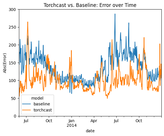
We can see that the torchcast model beats the baseline almost ever day. The clear exception is holidays (e.g. Thanksgiving and Christmas), which makes sense: we didn’t add any features for these to our torchcast model, while the baseline model essentially gets these for free. Future attempts could resolve this straightforwardly by adding dummy-features to our LinearModel, or by increasing the K (aka “wiggliness”) parameter (see “Encoding Seasonlity as Fourier Terms” above).
By Group
Now let’s compare over the whole test period, focusing on percent error (relative to that group’s average) so that we can weight small and large groups equally.
[34]:
from matplotlib.ticker import PercentFormatter

df_compare_per_group = (df_compare_long
                         .groupby(['group', 'dataset', 'model'])
                         [['error', 'kW']].mean()
                         .reset_index()
                         .assign(prop_error=lambda df: df['error'] / df['kW']))

compare_per_group_agg = (df_compare_per_group
                         .groupby(['dataset', 'model'])
                         .agg(prop_error=('prop_error', 'mean'), sem=('prop_error', 'sem')))

(compare_per_group_agg.loc['test']['prop_error']
 .plot(kind='bar',
       yerr=compare_per_group_agg.loc['test']['sem'],
       ylabel='Percent Error',
       title="Torchcast vs. Baseline: % Error in Test Set")
 .yaxis.set_major_formatter(PercentFormatter(xmax=1)))
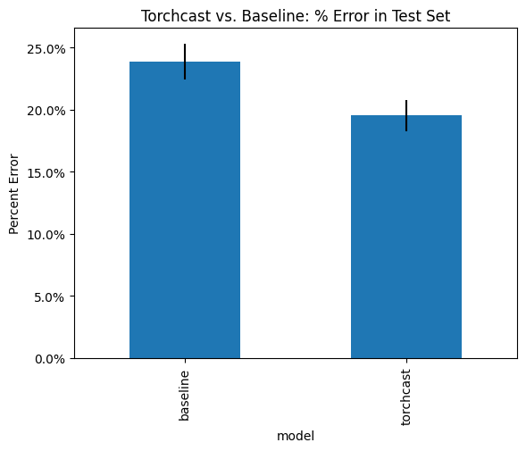
We see that the torchcast forecasts have significantly lower % error on average.