Quick Start
torchcast is a python package for time-series forecasting in PyTorch. Its focus is on training and forecasting with batches of time-serieses, rather than training separate models for one time-series at a time. In addition, it provides robust support for multivariate time-series, where multiple correlated measures are being forecasted.
To briefly provide an overview of these features, we’ll use a dataset from the UCI Machine Learning Data Repository. It includes data on air pollutants and weather from 12 sites.
[2]:
df_aq = load_air_quality_data('weekly')

df_aq
loading from gh...
[2]:
| week | station | PM2p5 | PM10 | SO2 | NO2 | CO | O3 | TEMP | PRES | DEWP | RAIN | WSPM | |
|---|---|---|---|---|---|---|---|---|---|---|---|---|---|
| 0 | 2013-02-25 | Aotizhongxin | 38.263889 | 57.791667 | 36.541667 | 56.750000 | 958.236111 | 37.583333 | 2.525000 | 1022.777778 | -15.666667 | 0.0 | 2.130556 |
| 1 | 2013-02-25 | Changping | 31.986111 | 47.152778 | 31.870773 | 44.969203 | 870.355072 | 45.925725 | 1.915278 | 1019.633333 | -16.231944 | 0.0 | 1.475000 |
| 2 | 2013-02-25 | Dingling | 28.083333 | 37.816919 | 15.955314 | 34.916667 | 627.838164 | 49.222222 | 1.915278 | 1019.633333 | -16.231944 | 0.0 | 1.475000 |
| 3 | 2013-02-25 | Dongsi | 45.083333 | 60.680556 | 31.687198 | 60.160024 | 1165.036836 | 43.635870 | 2.268056 | 1024.697222 | -16.913889 | 0.0 | 1.775000 |
| 4 | 2013-02-25 | Guanyuan | 38.472222 | 55.208333 | 35.467995 | 62.855676 | 1075.746981 | 38.277778 | 2.525000 | 1022.777778 | -15.666667 | 0.0 | 2.130556 |
| ... | ... | ... | ... | ... | ... | ... | ... | ... | ... | ... | ... | ... | ... |
| 2515 | 2017-02-27 | Nongzhanguan | 46.807359 | 76.195652 | 13.304348 | 56.108696 | 1032.608696 | 41.152174 | 9.647917 | 1016.014583 | -9.964583 | 0.0 | 1.787500 |
| 2516 | 2017-02-27 | Shunyi | 47.020833 | 58.625000 | 13.750000 | 61.791667 | 1033.333333 | 40.750000 | 8.289583 | 1016.695833 | -8.525000 | 0.0 | 1.827083 |
| 2517 | 2017-02-27 | Tiantan | 43.662500 | 70.429167 | 10.577273 | 64.052381 | 1012.954545 | 37.800000 | 9.647917 | 1016.014583 | -9.964583 | 0.0 | 1.787500 |
| 2518 | 2017-02-27 | Wanliu | 36.979167 | 60.750000 | 12.663949 | 65.371377 | 1061.322464 | 35.964015 | 8.868750 | 1014.450000 | -9.300000 | 0.0 | 1.558333 |
| 2519 | 2017-02-27 | Wanshouxigong | 39.550595 | 55.199405 | 9.835404 | 57.981366 | 993.788820 | 37.146998 | 9.647917 | 1016.014583 | -9.964583 | 0.0 | 1.787500 |
2520 rows × 13 columns
Prepare our Dataset
In torchcast we set up our data and model with the following:
The
groupswhich define separate time-serieses. Here we have multiple sites. Groups are not necessarily simultanoues to each other (e.g. we could have time-series of product purchases with products having varying release-dates) and correlations across these groups are not modeled.The
measureswhich define separate metrics we are measuring simultanously. Here we have the two kinds of particulate-matter (2.5 and 10).
The TimeSeriesDataset is similar to PyTorch’s native TensorDataset, with some useful metadata on the batch of time-serieses (the station names, the dates for each).
For a quick example, we’ll focus on predicting particulate-matter (PM2.5 and PM10). We’ll log-transform since this is strictly positive.
[3]:
df_aq['PM2p5_log10'] = np.log10(df_aq['PM2p5'])
df_aq['PM10_log10'] = np.log10(df_aq['PM10'])

# create a dataset:
dataset_all = TimeSeriesDataset.from_dataframe(
    dataframe=df_aq,
    dt_unit='W',
    measure_colnames=['PM2p5_log10', 'PM10_log10'],
    group_colname='station',
    time_colname='week'
)

# Split out training period:
SPLIT_DT = np.datetime64('2016-02-22')
dataset_train, _ = dataset_all.train_val_split(dt=SPLIT_DT)
dataset_train
[3]:
TimeSeriesDataset(sizes=[torch.Size([12, 156, 2])], measures=(('PM2p5_log10', 'PM10_log10'),))
Specify our Model
In torchcast our forecasting model is defined by measures and processes. The processes give rise to the measure-able behavior. Here we’ll specify a random-walk/trend component and a yearly seasonal component for each pollutant.
[4]:
processes = []
for m in dataset_train.measures[0]:
    processes.extend([
        LocalTrend(id=f'{m}_trend', measure=m),
        Season(id=f'{m}_day_in_year', period=365.25 / 7, dt_unit='W', K=3, measure=m, fixed=True)
    ])
kf_first = KalmanFilter(measures=dataset_train.measures[0], processes=processes)
Train our Model
The KalmanFilter class provides a convenient fit() method that’s useful for avoiding standard boilerplate for full-batch training:
[5]:
kf_first.fit(
    dataset_train.tensors[0],
    start_offsets=dataset_train.start_datetimes
)
For measure PM2p5_log10, setting initial value by setting 'PM2p5_log10_trend.position' to 1.8531
For measure PM10_log10, setting initial value by setting 'PM10_log10_trend.position' to 1.9870
[5]:
KalmanFilter(
  (measure_covariance): Covariance()
  (processes): ModuleDict(
    (PM2p5_log10_trend): LocalTrend(id='PM2p5_log10_trend', measure='PM2p5_log10')
    (PM2p5_log10_day_in_year): Season(id='PM2p5_log10_day_in_year', measure='PM2p5_log10')
    (PM10_log10_trend): LocalTrend(id='PM10_log10_trend', measure='PM10_log10')
    (PM10_log10_day_in_year): Season(id='PM10_log10_day_in_year', measure='PM10_log10')
  )
  (process_covariance): Covariance()
  (initial_covariance): Covariance()
)
Calling forward() on our KalmanFilter produces a Predictions object. If you’re writing your own training loop, you’d simply use the log_prob() method as the loss function:
[6]:
pred = kf_first(
        dataset_train.tensors[0],
        start_offsets=dataset_train.start_datetimes,
        out_timesteps=dataset_all.tensors[0].shape[1]
)

loss = -pred.log_prob(dataset_train.tensors[0]).mean()
print(loss)
tensor(-0.7386, grad_fn=<NegBackward0>)
Inspect & Visualize our Output
Predictions can easily be converted to Pandas DataFrames for ease of inspecting predictions, comparing them to actuals, and visualizing:
[7]:
df_pred = pred.to_dataframe(dataset_all)
df_pred[['actual','mean','upper','lower']] = 10 ** df_pred[['actual','mean','upper','lower']]
df_pred
[7]:
| mean | lower | upper | actual | group | time | measure | |
|---|---|---|---|---|---|---|---|
| 0 | 92.422127 | 36.691303 | 232.803177 | 38.263885 | Aotizhongxin | 2013-02-25 | PM2p5_log10 |
| 1 | 90.387688 | 35.971073 | 227.125061 | 139.428558 | Aotizhongxin | 2013-03-04 | PM2p5_log10 |
| 2 | 87.031174 | 34.662758 | 218.517685 | 157.071411 | Aotizhongxin | 2013-03-11 | PM2p5_log10 |
| 3 | 86.160835 | 34.325199 | 216.275192 | 67.321434 | Aotizhongxin | 2013-03-18 | PM2p5_log10 |
| 4 | 83.725342 | 33.348335 | 210.203384 | 107.333313 | Aotizhongxin | 2013-03-25 | PM2p5_log10 |
| ... | ... | ... | ... | ... | ... | ... | ... |
| 205 | 91.582069 | 40.944695 | 204.844025 | 119.059532 | Wanshouxigong | 2017-01-30 | PM10_log10 |
| 206 | 94.056496 | 41.974403 | 210.762299 | 61.144417 | Wanshouxigong | 2017-02-06 | PM10_log10 |
| 207 | 97.202370 | 43.294636 | 218.232605 | 139.613068 | Wanshouxigong | 2017-02-13 | PM10_log10 |
| 208 | 100.741608 | 44.783207 | 226.622269 | 47.162453 | Wanshouxigong | 2017-02-20 | PM10_log10 |
| 209 | 104.334366 | 46.292297 | 235.150543 | 55.199409 | Wanshouxigong | 2017-02-27 | PM10_log10 |
5040 rows × 7 columns
[8]:
df_pred['percent_error'] = np.abs(df_pred['mean'] - df_pred['actual']) / df_pred['actual']
print("Percent Error: {:.1%}".format(df_pred.query("time>@SPLIT_DT")['percent_error'].mean()))
Percent Error: 35.5%
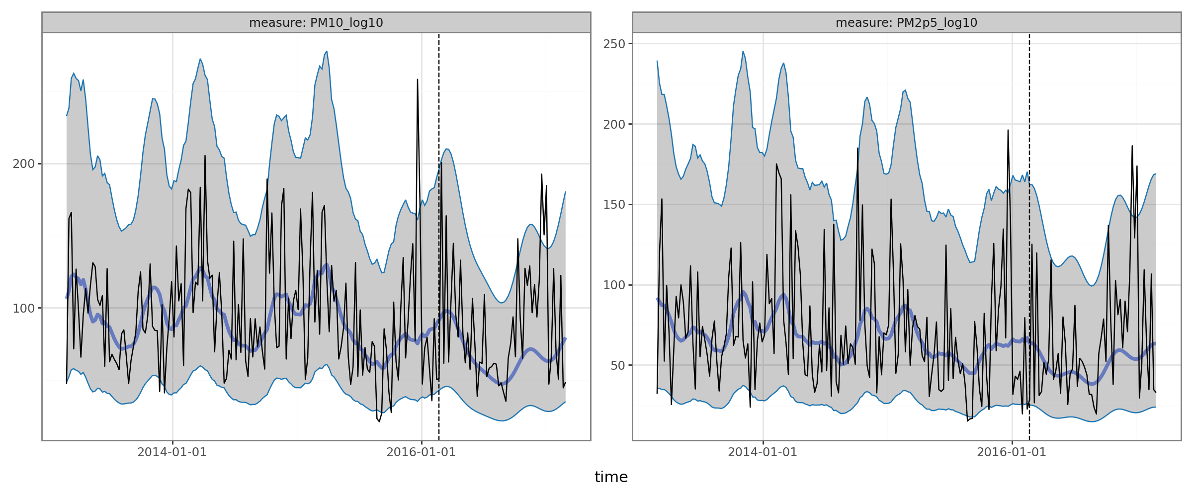
The Predictions class comes with a plot classmethod for getting simple plots of forecasted vs. actual:
[9]:
pred.plot(df_pred.query("group=='Changping'"), split_dt=SPLIT_DT, time_colname='time', group_colname='group')
[9]:
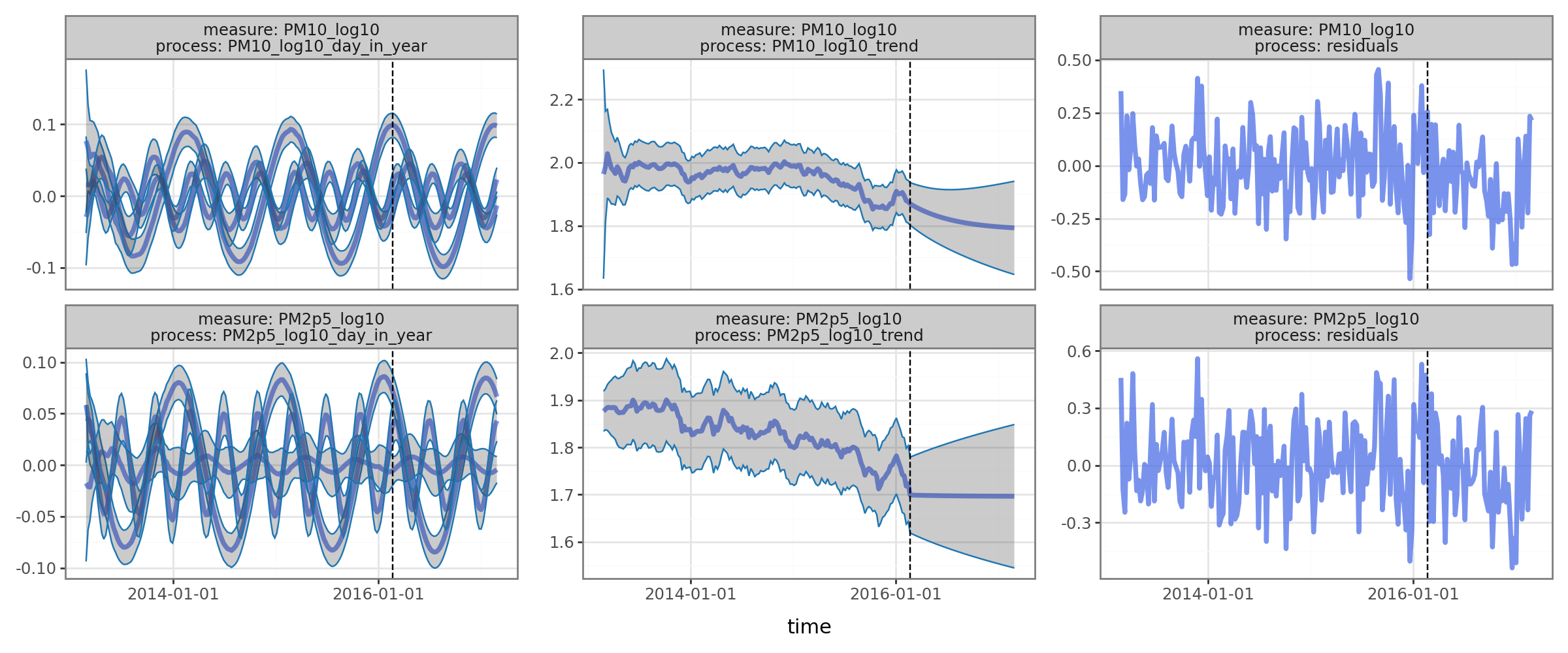
Finally you can produce dataframes that decompose the predictions into the underlying processes that produced them:
[10]:
pred.plot(
    pred.to_dataframe(dataset_all, type='observed_states').query("group=='Changping'"), split_dt=SPLIT_DT,
    time_colname='time', group_colname='group'
)
[10]:
[ ]: