Multivariate Forecasts: Beijing Multi-Site Air-Quality Data
We’ll demonstrate several features of torchcast using a dataset from the UCI Machine Learning Data Repository. It includes data on air pollutants and weather from 12 sites.
[3]:
df_aq = load_air_quality_data('daily')

SPLIT_DT = np.datetime64('2016-02-22')
df_aq['dataset'] = np.where(df_aq['date'] > SPLIT_DT, 'val', 'train')
df_aq
[3]:
| date | station | PM2p5 | PM10 | SO2 | NO2 | CO | O3 | TEMP | PRES | DEWP | RAIN | WSPM | dataset | |
|---|---|---|---|---|---|---|---|---|---|---|---|---|---|---|
| 0 | 2013-03-01 | Aotizhongxin | 7.125000 | 10.750000 | 11.708333 | 22.583333 | 429.166667 | 63.875000 | 1.391667 | 1026.875000 | -18.745833 | 0.0 | 3.254167 | train |
| 1 | 2013-03-01 | Changping | 5.083333 | 18.958333 | 16.041667 | 15.333333 | 387.500000 | 77.791667 | 0.812500 | 1023.858333 | -19.583333 | 0.0 | 2.133333 | train |
| 2 | 2013-03-01 | Dingling | 6.375000 | 6.409091 | 3.000000 | 2.625000 | 204.166667 | 81.958333 | 0.812500 | 1023.858333 | -19.583333 | 0.0 | 2.133333 | train |
| 3 | 2013-03-01 | Dongsi | 6.416667 | 9.875000 | 8.478261 | 28.521739 | 395.652174 | 72.782609 | 1.325000 | 1028.783333 | -21.466667 | 0.0 | 3.308333 | train |
| 4 | 2013-03-01 | Guanyuan | 7.541667 | 11.666667 | 8.500000 | 28.500000 | 400.000000 | 63.166667 | 1.391667 | 1026.875000 | -18.745833 | 0.0 | 3.254167 | train |
| ... | ... | ... | ... | ... | ... | ... | ... | ... | ... | ... | ... | ... | ... | ... |
| 17527 | 2017-02-28 | Nongzhanguan | 17.523810 | 24.739130 | 7.347826 | 35.652174 | 526.086957 | 56.086957 | 10.958333 | 1014.887500 | -12.783333 | 0.0 | 2.058333 | val |
| 17528 | 2017-02-28 | Shunyi | 20.708333 | 28.500000 | 7.125000 | 39.666667 | 579.166667 | 57.291667 | 9.250000 | 1015.550000 | -10.429167 | 0.0 | 2.025000 | val |
| 17529 | 2017-02-28 | Tiantan | 14.875000 | 32.708333 | 6.454545 | 42.904762 | 540.909091 | 57.600000 | 10.958333 | 1014.887500 | -12.783333 | 0.0 | 2.058333 | val |
| 17530 | 2017-02-28 | Wanliu | 9.958333 | 25.583333 | 7.458333 | 40.916667 | 479.166667 | 54.791667 | 10.516667 | 1013.345833 | -12.266667 | 0.0 | 1.800000 | val |
| 17531 | 2017-02-28 | Wanshouxigong | 10.958333 | 21.541667 | 4.956522 | 31.391304 | 530.434783 | 54.913043 | 10.958333 | 1014.887500 | -12.783333 | 0.0 | 2.058333 | val |
17532 rows × 14 columns
Univariate Forecasts
Let’s build a model to predict total particulate-matter (PM2.5 and PM10).
First, we’ll make our target the sum of these two types. We’ll log-transform since this is strictly positive.
[4]:
df_aq['PM'] = df_aq['PM10'] + df_aq['PM2p5']
df_aq['PM_log10'] = np.log10(df_aq['PM'])
[5]:
# create our dataset:
dataset_pm = TimeSeriesDataset.from_dataframe(
    dataframe=df_aq,
    dt_unit='D',
    measure_colnames=['PM_log10'],
    group_colname='station',
    time_colname='date'
)
dataset_pm_train, _ = dataset_pm.train_val_split(dt=SPLIT_DT)
[6]:
# specify our model:
from torchcast.process import LocalTrend, Season

kf_pm = KalmanFilter(
    measures=['PM_log10'],
    processes=[
        LocalTrend(id='trend'),
        Season(
            id='day_in_year',
            period=365.25,
            dt_unit='D',
            K=4,
            fixed=True
        ),
        Season(
            id='day_in_week',
            period=7,
            dt_unit='D',
            K=2,
            fixed=True
        )
    ],
)
[7]:
# fit it:
kf_pm.fit(
    dataset_pm_train.tensors[0],
    start_offsets=dataset_pm_train.start_datetimes,
    n_step=5, every_step=False,
)
For measure PM_log10, setting initial value by setting 'trend.position' to 2.1530
[7]:
KalmanFilter(
  (measure_covariance): Covariance()
  (processes): ModuleDict(
    (trend): LocalTrend(id='trend', measure='PM_log10')
    (day_in_year): Season(id='day_in_year', measure='PM_log10')
    (day_in_week): Season(id='day_in_week', measure='PM_log10')
  )
  (process_covariance): Covariance()
  (initial_covariance): Covariance()
)
The n_step argument
When fitting our model, we use the n_step argument to improve longer-range forecasts. We know we will be using our model to forecast weeks/months into the future, so we ‘encourage’ the model to get good at this task by optimizing for 5-step-ahead forecasts (rather than the traditional 1-step-ahead forecasts) in training.
This simple strategy can often dramatically improve the quality of long-range forecasts; and paired with the every_step=False setting, does not cause an increase in training-time.
Let’s see how our forecasts look:
[8]:
# helper for transforming log back to original:
def inverse_transform(df: pd.DataFrame) -> pd.DataFrame:
    df = df.copy()
    # bias-correction for log-transform (see https://otexts.com/fpp2/transformations.html#bias-adjustments)
    df['mean'] = df['mean'] + .5 * df['std'] ** 2
    df['lower'] = df['mean'] - 1.96 * df['std']
    df['upper'] = df['mean'] + 1.96 * df['std']
    # inverse the log10:
    df[['actual', 'mean', 'upper', 'lower']] = 10 ** df[['actual', 'mean', 'upper', 'lower']]
    df['measure'] = df['measure'].str.replace('_log10', '')
    return df
[9]:
# generate forecasts:
forecast = kf_pm(
        dataset_pm_train.tensors[0],
        start_offsets=dataset_pm_train.start_datetimes,
        out_timesteps=dataset_pm.tensors[0].shape[1]
)

# convert to dataframe, back-transform:
df_uv_pred = (forecast
             .set_metadata(group_colname='station', time_colname='date')
             .to_dataframe(dataset_pm, conf=None)
             .pipe(inverse_transform))

# plot:
forecast.plot(
    df_uv_pred.query("date>'2014-01-01'").query("station.isin(['Aotizhongxin', 'Dingling'])"),
    max_num_groups=2,
    split_dt=SPLIT_DT,
    figure_size=(6,5)
) #+ scale_y_log10()
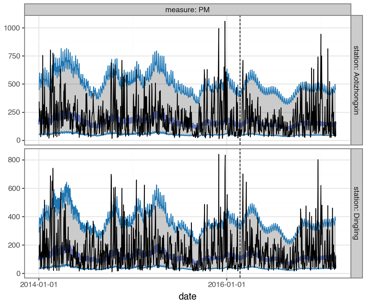
Multivariate Forecasts
Can we improve our model by splitting the pollutant we are forecasting into its two types (2.5 and 10), and modeling them in a multivariate manner?
[10]:
# create a dataset:
df_aq['PM10_log10'] = np.log10(df_aq['PM10'])
df_aq['PM2p5_log10'] = np.log10(df_aq['PM2p5'])
dataset_pm_mv = TimeSeriesDataset.from_dataframe(
    dataframe=df_aq,
    dt_unit='D',
    measure_colnames=['PM10_log10','PM2p5_log10'],
    group_colname='station',
    time_colname='date'
)
dataset_pm_mv_train, _ = dataset_pm_mv.train_val_split(dt=SPLIT_DT)

# create a model:
_processes = []
for m in dataset_pm_mv.measures[0]:
    _processes.extend([
        LocalTrend(id=f'{m}_trend', measure=m),
        Season(
            id=f'{m}_day_in_year',
            period=365.25,
            dt_unit='D',
            K=4,
            measure=m,
            fixed=True
        ),

        Season(
            id=f'{m}_day_in_week',
            period=7,
            dt_unit='D',
            K=2,
            measure=m,
            fixed=True
        )
    ])
kf_pm_mv = KalmanFilter(
    measures=dataset_pm_mv.measures[0],
    processes=_processes,
)

# fit:
kf_pm_mv.fit(
    dataset_pm_mv_train.tensors[0],
    start_offsets=dataset_pm_mv_train.start_datetimes,
    n_step=5, every_step=False,
)
For measure PM10_log10, setting initial value by setting 'PM10_log10_trend.position' to 1.9197
For measure PM2p5_log10, setting initial value by setting 'PM2p5_log10_trend.position' to 1.7518
[10]:
KalmanFilter(
  (measure_covariance): Covariance()
  (processes): ModuleDict(
    (PM10_log10_trend): LocalTrend(id='PM10_log10_trend', measure='PM10_log10')
    (PM10_log10_day_in_year): Season(id='PM10_log10_day_in_year', measure='PM10_log10')
    (PM10_log10_day_in_week): Season(id='PM10_log10_day_in_week', measure='PM10_log10')
    (PM2p5_log10_trend): LocalTrend(id='PM2p5_log10_trend', measure='PM2p5_log10')
    (PM2p5_log10_day_in_year): Season(id='PM2p5_log10_day_in_year', measure='PM2p5_log10')
    (PM2p5_log10_day_in_week): Season(id='PM2p5_log10_day_in_week', measure='PM2p5_log10')
  )
  (process_covariance): Covariance()
  (initial_covariance): Covariance()
)
Generate our forecasts as before:
[11]:
with torch.no_grad():
    forecast_mv = kf_pm_mv(
        dataset_pm_mv_train.tensors[0],
        start_offsets=dataset_pm_mv_train.start_datetimes,
        out_timesteps=dataset_pm_mv.num_timesteps # <--- how we ask it to forecast past original times
    )
forecast_mv.means.shape
[11]:
torch.Size([12, 1461, 2])
[12]:
forecast_mv.plot(
    forecast_mv
    .set_metadata(group_colname='station', time_colname='date')
    .to_dataframe(dataset_pm_mv, conf=None)
    .pipe(inverse_transform)
    .query("date>'2014-01-01'"),
    max_num_groups=2,
    split_dt=SPLIT_DT,
)
Subsetting to groups: ['Aotizhongxin', 'Dingling']
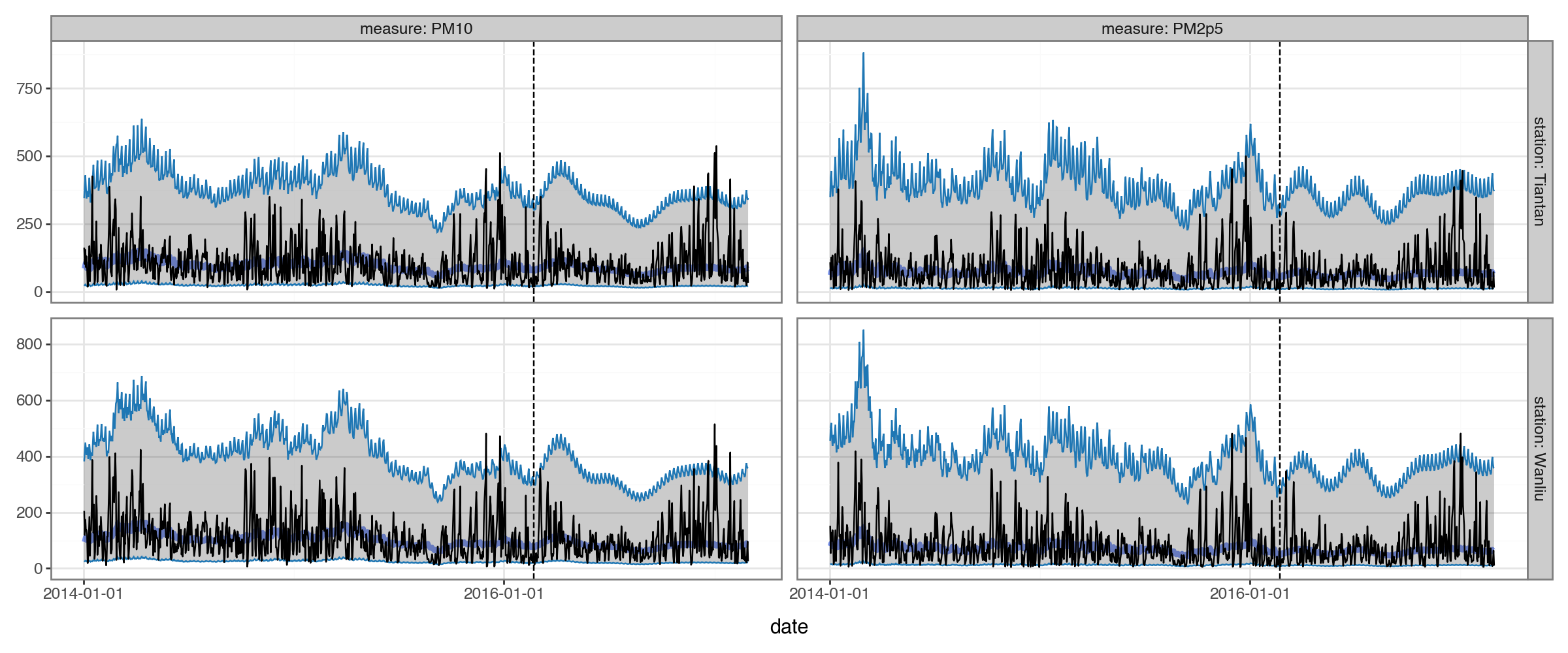
At this point, though, we run into a problem: we we have forecasts for both PM2.5 and PM10, but we ultimately want a forecast for their sum. With untransformed data, we could take advantage of the fact that sum of correlated normals is still normal; but we have log-transformed our measures. This seems like it was the right choice (i.e. our residuals look reasonably normal and i.i.d):
[13]:
forecast_mv.plot(
    forecast_mv
    .to_dataframe(dataset_pm_mv, type='components')
    .query("process=='residuals'")
    .query("date>'2014-01-01'"),
    figure_size=(6,5)
) + facet_wrap('measure', ncol=1)
Subsetting to groups: ['Wanliu']
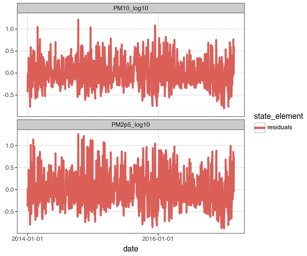
In this case, we can’t take the sum of our forecasts to get the forecast of the sum, and there’s no simple closed-form expression for the sum of lognormals.
One option that is fairly easy in torchcast is to use a Monte-Carlo approach: we’ll just generate random-samples based on the means and covariances underlying our forecast. In that case, the sum of the PM2.5 + PM10 forecasted-samples is the forecasted PM sum we are looking for:
[14]:
@torch.no_grad()
def sum_mc_preds_as_df(preds: Predictions,
                          dataset: TimeSeriesDataset,
                          inverse_transform_fun: callable,
                          num_draws: int = 1000,
                          **kwargs) -> pd.DataFrame:
    """
    Our predictions are on the transformed scale, and we'd like to sum across measures on the original scale;
    this function uses a monte-carlo approach to do this.
    """
    # generate draws from the forecast distribution, apply inverse-transform:
    mean, cov = preds
    eps = 1e-6 * torch.eye(cov.shape[-1]).unsqueeze(0).unsqueeze(0) # handle numerical instability
    mc_draws = torch.distributions.MultivariateNormal(mean, cov + eps, validate_args=False).rsample((num_draws,))
    # sum across measures (e.g. 2.5 and 10), then mean across draws:
    mc_predictions = inverse_transform_fun(mc_draws).sum(-1, keepdim=True).mean(0)
    # convert to a dataframe
    return TimeSeriesDataset.tensor_to_dataframe(
        mc_predictions,
        times=dataset.times(),
        group_names=dataset.group_names,
        measures=['predicted'],
        **kwargs
    )
[15]:
df_mv_pred = sum_mc_preds_as_df(
    forecast_mv,
    dataset_pm_mv,
    inverse_transform_fun=lambda x: 10 ** x,
    group_colname='station',
    time_colname='date'
)
df_mv_pred.head()
[15]:
| predicted | station | date | |
|---|---|---|---|
| 0 | 287.592163 | Aotizhongxin | 2013-03-01 |
| 1 | 153.595001 | Aotizhongxin | 2013-03-02 |
| 2 | 243.020874 | Aotizhongxin | 2013-03-03 |
| 3 | 231.288498 | Aotizhongxin | 2013-03-04 |
| 4 | 339.382141 | Aotizhongxin | 2013-03-05 |
Evaluating Performance
[16]:
def get_station_error(df: pd.DataFrame, pred_colname: str = 'mean', actual_colname: str = 'actual') -> pd.DataFrame:
    return (df
             .assign(sq_error=lambda df: (df[pred_colname] - df[actual_colname]) ** 2)
             .groupby(['station'])
             ['sq_error'].mean()
             .reset_index()
             .assign(rmse= lambda df: df['sq_error'] ** .5))

def agg_within_group_err(df: pd.DataFrame, error_col : str = 'rmse', group_col: str = 'station') -> pd.DataFrame:
    df = df.copy(deep=False)
    df['error_norm'] = df[error_col] - df.groupby(group_col)[error_col].transform('mean')
    return df.groupby('model').agg(**{error_col : (error_col, 'mean'), 'sem' : ('error_norm', 'sem')})
[17]:
df_fct_err = pd.concat([
            df_uv_pred
             .loc[lambda df: df['date'] > SPLIT_DT,:]
             .pipe(get_station_error)
             .assign(model='univariate')
            ,
            df_mv_pred
             .loc[lambda df: df['date'] > SPLIT_DT,:]
             .merge(df_aq.loc[:, ['station', 'date', 'PM']])
             .pipe(get_station_error, pred_colname='predicted', actual_colname='PM')
             .assign(model='multivariate')
]).reset_index(drop=True)
df_fct_err.sort_values('station').tail(6)
[17]:
| station | sq_error | rmse | model | |
|---|---|---|---|---|
| 21 | Tiantan | 22168.937549 | 148.892369 | multivariate |
| 9 | Tiantan | 24113.337891 | 155.284698 | univariate |
| 22 | Wanliu | 20048.709105 | 141.593464 | multivariate |
| 10 | Wanliu | 21591.140625 | 146.939240 | univariate |
| 11 | Wanshouxigong | 25694.980469 | 160.296539 | univariate |
| 23 | Wanshouxigong | 23840.210635 | 154.402755 | multivariate |
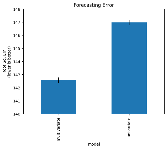
Below we aggregate the performance across stations (controlling for within-station variation to reduce noise).
We see the multivariate approach outperforms the univariate one despite the fact that we are just comparing univariate forecasts! That is, modeling the two types of PM with a multivariate approach was better for predicting their total than simply modeling that total directly.
[18]:
df_fct_err_agg = agg_within_group_err(df_fct_err)

# https://chris-said.io/2014/12/01/independent-t-tests-and-the-83-confidence-interval-a-useful-trick-for-eyeballing-your-data/
from scipy import stats
sem_multi = -stats.norm.ppf((1 - .83) / 2)

df_fct_err_agg['rmse'].plot(
    kind='bar',
    yerr=df_fct_err_agg['sem'] * sem_multi,
    ylabel="Root Sq. Err\n(lower is better)",
    title="Forecasting Error",
    ylim=(140,150)
)
plt.show()
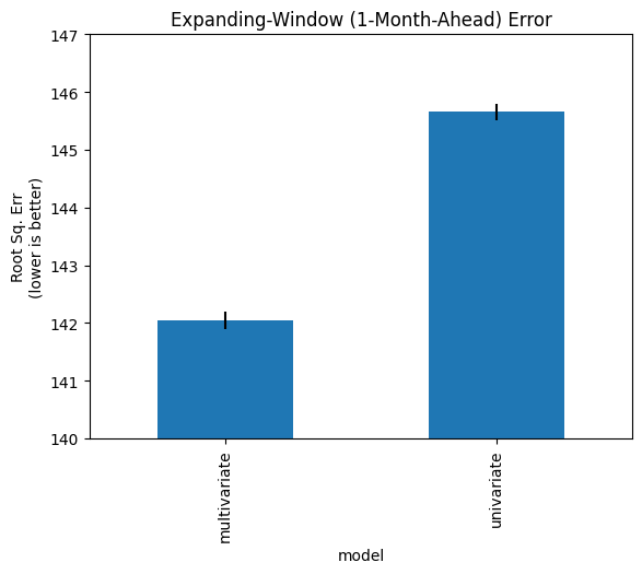
Expanding Window Approach
One limitation to evaluating performance with a single train/val split-date is we run the risk that our results are sensitive to that particular split.
An alternative approach is an “expanding window”: we loop over the series, training on increasingly long sections, and forecasting on a fixed period beyond this. For short series, it might make sense to retrain on each iteration.
However for longer series, to speed up the process, we might want to simply use a particular date-range for training, then do our expanding window procedure on the held out remainder. (This is challenging in many forecasting APIs because they do not allow passing new series – or extensions of the trained series – at inference time, but instead require retraining.)
In torchcast, it’s easy to apply an expanding-window method with the n_step argument, avoiding the need for any refit -> forecast external loop.
[19]:
with torch.no_grad():
    one_mo_uv = kf_pm(
        dataset_pm.tensors[0],
        start_offsets=dataset_pm.start_datetimes,
        n_step=30
    )
    one_mo_mv = kf_pm_mv(
        dataset_pm_mv.tensors[0],
        start_offsets=dataset_pm_mv.start_datetimes,
        n_step=30
    )

df_backtest_err1mo = pd.concat([

    one_mo_uv
    .to_dataframe(dataset_pm, time_colname='date', group_colname='station', conf=None)
    .pipe(inverse_transform)
    .loc[lambda df: df['date'] > SPLIT_DT, :]
    .pipe(get_station_error)
    .assign(model='univariate')
    ,

    sum_mc_preds_as_df(one_mo_mv,
                          dataset_pm_mv,
                          inverse_transform_fun=lambda x: 10 ** x,
                          group_colname='station',
                          time_colname='date')
    .loc[lambda df: df['date'] > SPLIT_DT,:]
    .merge(df_aq[['station', 'date', 'PM']])
    .pipe(get_station_error, pred_colname='predicted', actual_colname='PM')
    .assign(model='multivariate')
])

df_backtest1mo_err_agg = agg_within_group_err(df_backtest_err1mo)

df_backtest1mo_err_agg['rmse'].plot(
    kind='bar',
    yerr=df_backtest1mo_err_agg['sem'],
    ylabel="Root Sq. Err\n(lower is better)",
    title="Expanding-Window (1-Month-Ahead) Error",
    ylim=(140,148)
)
plt.show()
Adding Predictors
In many settings we have external (a.k.a. exogenous) predictors we’d like to incorporate. Here we’ll use four predictors corresponding to weather conditions. Of course, in a forecasting context, we run into the problem of needing to fill in values for these predictors for future dates. For an arbitrary forecast horizon this can be a complex issue; for simplicity here we’ll focus on the 4-week-ahead predictions we used above, and simply lag our weather predictors by 4.
[20]:
from torchcast.process import LinearModel

# prepare external predictors:
predictors_raw = ['TEMP', 'PRES', 'DEWP']
predictors = [p.lower() + '_lag30' for p in predictors_raw]
# standardize:
predictor_means = df_aq.query("dataset=='train'")[predictors_raw].mean()
predictor_stds = df_aq.query("dataset=='train'")[predictors_raw].std()
df_aq[predictors] = (df_aq[predictors_raw] - predictor_means) / predictor_stds
# lag:
df_aq[predictors] = df_aq.groupby('station')[predictors].shift(30, fill_value=0)

# create dataset:
dataset_pm_lm = TimeSeriesDataset.from_dataframe(
    dataframe=df_aq,
    dt_unit='D',
    y_colnames=['PM10_log10','PM2p5_log10'],
    X_colnames=predictors,
    group_colname='station',
    time_colname='date',
)
dataset_pm_lm_train, _ = dataset_pm_lm.train_val_split(dt=SPLIT_DT)
dataset_pm_lm_train
[20]:
TimeSeriesDataset(sizes=[torch.Size([12, 1088, 2]), torch.Size([12, 1088, 3])], measures=(('PM10_log10', 'PM2p5_log10'), ('temp_lag30', 'pres_lag30', 'dewp_lag30')))
[21]:
_processes = []
for m in dataset_pm_lm.measures[0]:
    _processes.extend([
        LocalTrend(id=f'{m}_trend', measure=m),

        Season(
            id=f'{m}_day_in_year',
            period=365.25,
            dt_unit='D',
            K=4,
            measure=m,
            fixed=True
        ),

        Season(
            id=f'{m}_day_in_week',
            period=7,
            dt_unit='D',
            K=2,
            measure=m,
            fixed=True
        ),


        LinearModel(
            id=f'{m}_lm',
            predictors=predictors,
            measure=m
        )
    ])
kf_pm_lm = KalmanFilter(
    measures=dataset_pm_lm.measures[0], processes=_processes
)
[22]:
# fit:
y, X = dataset_pm_lm_train.tensors
kf_pm_lm.fit(
    y,
    X=X, # if you want to supply different predictors to different processes, you can use `{process_name}__X`
    start_offsets=dataset_pm_lm_train.start_datetimes,
    n_step=5,
    every_step=False
)
For measure PM10_log10, setting initial value by setting 'PM10_log10_trend.position' to 1.9197
For measure PM2p5_log10, setting initial value by setting 'PM2p5_log10_trend.position' to 1.7518
[22]:
KalmanFilter(
  (measure_covariance): Covariance()
  (processes): ModuleDict(
    (PM10_log10_trend): LocalTrend(id='PM10_log10_trend', measure='PM10_log10')
    (PM10_log10_day_in_year): Season(id='PM10_log10_day_in_year', measure='PM10_log10')
    (PM10_log10_day_in_week): Season(id='PM10_log10_day_in_week', measure='PM10_log10')
    (PM10_log10_lm): LinearModel(id='PM10_log10_lm', measure='PM10_log10')
    (PM2p5_log10_trend): LocalTrend(id='PM2p5_log10_trend', measure='PM2p5_log10')
    (PM2p5_log10_day_in_year): Season(id='PM2p5_log10_day_in_year', measure='PM2p5_log10')
    (PM2p5_log10_day_in_week): Season(id='PM2p5_log10_day_in_week', measure='PM2p5_log10')
    (PM2p5_log10_lm): LinearModel(id='PM2p5_log10_lm', measure='PM2p5_log10')
  )
  (process_covariance): Covariance()
  (initial_covariance): Covariance()
)
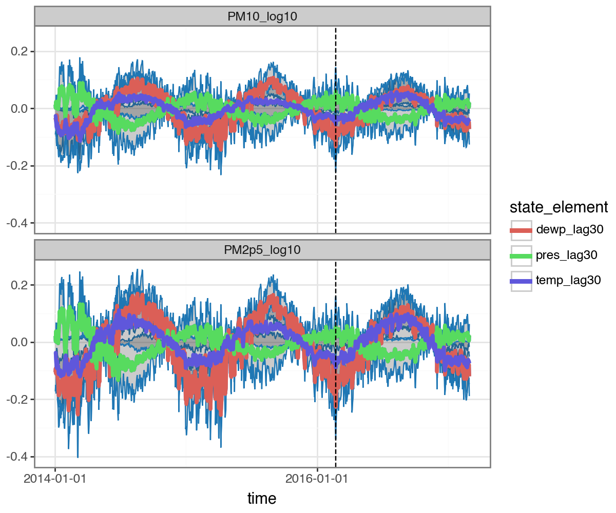
Here we show how to inspect the influence of each predictor:
[23]:
# inspect components:
with torch.no_grad():
    y, X = dataset_pm_lm.tensors
    one_mo_lm = kf_pm_lm(
        y,
        X=X,
        start_offsets=dataset_pm_lm.start_datetimes,
        n_step=30
    )
one_mo_lm.plot(
    one_mo_lm
    .to_dataframe(dataset_pm_lm, type='components')
    .query("process.str.contains('lm')")
    .query("time > '2014-01-01'"),
    split_dt=SPLIT_DT,
    figure_size=(6,5)
) + facet_wrap('measure', ncol=1)
Subsetting to groups: ['Wanshouxigong']
Re-Evaluate Performance
Now let’s look at the change in error from our earlier multivariate model vs. one that includes predictors.
We can’t compare the forecasts, since we have a fixed lag on our predictors. But we can easily compare the expanding-window results:
[24]:
df_backtest1mo_err_agg2 = agg_within_group_err(
    pd.concat([
        # old ones:
        df_backtest_err1mo,
        # new one:
        sum_mc_preds_as_df(one_mo_lm,
                              dataset_pm_lm,
                              inverse_transform_fun=lambda x: 10 ** x,
                              group_colname='station',
                              time_colname='date')
        .loc[lambda df: df['date'] > SPLIT_DT,:]
        .merge(df_aq[['station', 'date', 'PM']])
        .pipe(get_station_error, pred_colname='predicted', actual_colname='PM')
        .assign(model='mv_with_preds')
    ])
)

df_backtest1mo_err_agg2['rmse'].plot(
    kind='bar',
    yerr=df_backtest1mo_err_agg2['sem'] * sem_multi,
    ylabel="Root Sq. Err\n(lower is better)",
    title="Backtesting (1-Month-Ahead) Error",
    ylim=(140,148)
)
plt.show()
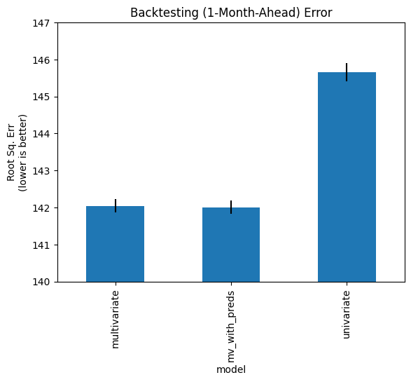
We see that the lagged predictors do not significantly impact performance.